

Informed Spatial Filtering for Sound Extraction using Distributed Microphone Arrays
Maja Taseska and Emanuel A. P. Habets
Published in IEEE/ACM Transactions on Audio, Speech and Language Processing Volume 22, Issue 7, July 2014, Pages 1195-1207
Problem description
Informed spatial filters (ISFs) are data-dependent filters which use almost instantaneous parametric information about the sound field to estimate the SOS of the different signals. In this work, we demonstrate the applicability of ISFs to the problem of blind source separation (BSS). BSS is achieved by computing an ISF for each source, which extracts the selected source while reducing the remaining sources and the background noise.
To compute such ISFs, the SOS of the different source signals and the background noise are required. As we process the signals in the frequency domain, the relevant SOS are given by the power spectral density (PSD) matrices of the different signals. Estimation of the PSD matrices is extremely challenging in practice where multiple sources are active simultaneously. The sparsity of speech signals in the short-time Fourier transform domain is exploited for PSD matrix estimation of simultaneously active sources. If each TF bin can be associated to the dominant source at that TF bin, the PSD matrix of a particular source can be obtained by temporal averaging across the bins that are associated to that source.
Hence, the main requirement for estimation of the PSD matrices is accurate association of the TF bins to sources, which in the BSS application, represents an unsupervised clustering problem. We perform clustering using the expectation-maximization algorithm applied to narrowband position estimates obtained from short time segments, where each of the sources of interest is active for a short period of time (2 seconds suffice, as shown in the examples below).
Further details about the problem, the proposed framework, and related research in the area can be found in the paper.
Setup and Signals
Setup
Measurements were carried out in a room with T60≈250 ms and dimensions 3.2×3.3×2.8 m. The sound scene was captured with two circular arrays with three DPA miniature microphones each, diameter 3 cm and inter-array distance 1.16 m. The source constellations and the room are illustrated in the respective examples below. The room impulse responses (RIRs) for each source-microphone pair were measured, where the signals were emitted by GENELEC loudspeakers at the locations of the sources. In addition, the RIRs for four loudspeakers facing the walls at the room corners were measured, and these impulse responses were used to create approximately diffuse background noise.
Signals
The microphone signals used to create the demos were obtained as follows
- Convolve clean speech signals with the measured RIRs at the source locations.
- Convolve babble noise signals with the measured RIRs for the loudspeakers facing the walls, sum the different babble signals together, scale them to achieve a desired diffuse-signal-to-noise ratio and add them together with the speech signals.
- Finally, add the measured sensor noise, scaled such that the signal-to-sensor-noise-ratio equals 30 dB.
The sampling frequency for all experiments was 16 kHz and the frame length of the short-time Fourier transform was L = 512 samples, with 50% overlap. Further details about the measurements and the performance evaluation can be found in the paper.
In the examples below first you can listen to the audio signal which was used to localize the sources and cluster the narrowband position estimates. We refer to this as the training period. Then the iterations of the EM algorithm and the learned clusters are illustrated. Finally, you can listen to the separated source signals.
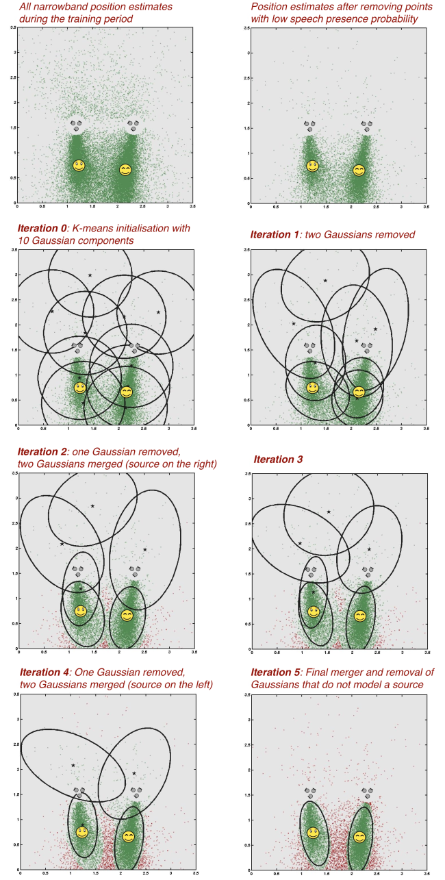
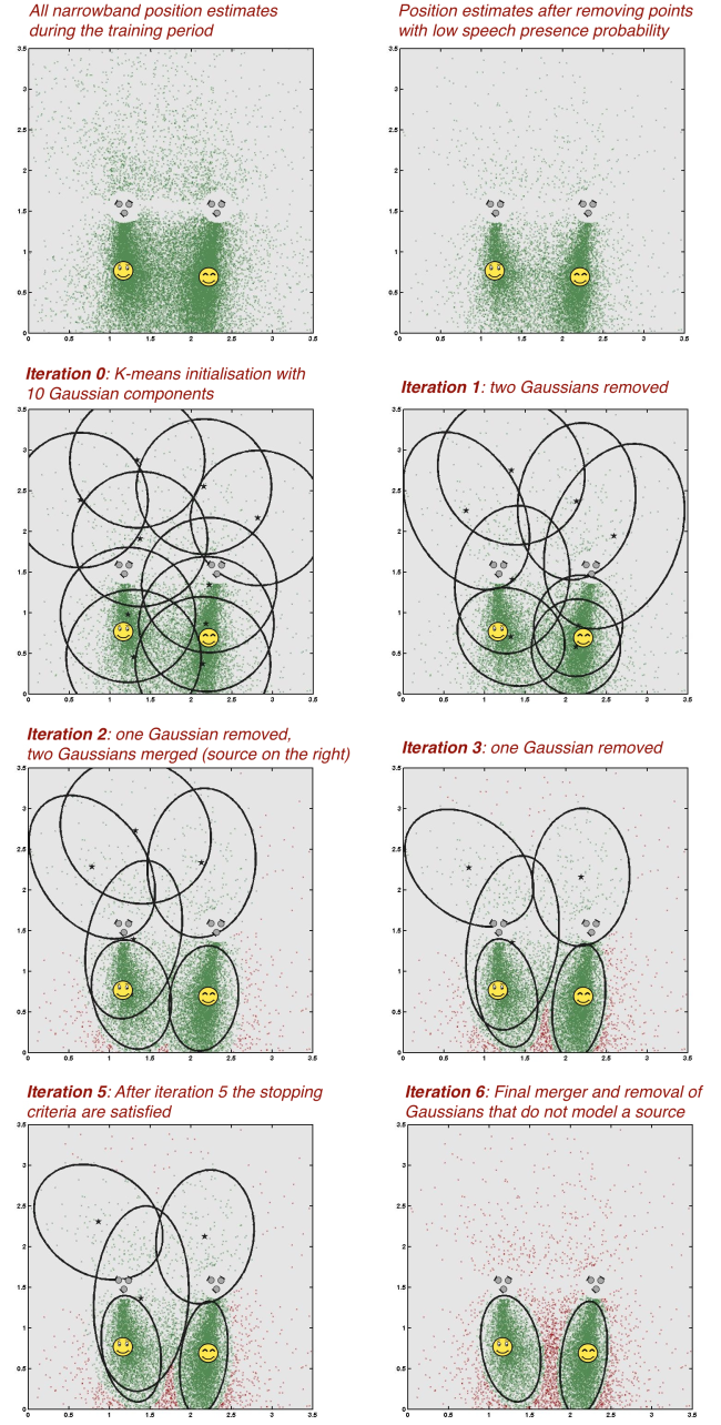
EXAMPLE 1
Two simultaneously active sources and background babble noise are captured by the microphone arrays. The training is performed using a 4.5 seconds segment where both sources are active. Two different noise conditions are tested, as given below.
Note that besides the significant difference in the noise level, the algorithm localizes the sources without notable performance degradation. The only difference is a slightly larger cluster variance, and one more required iteration in the case with lower signal-to-noise ratio.
A) Test under high signal to noise ratio, 23 dB with respect to the sum of speech signals.
- Listen to the portion of the signal used for training by hitting the start button below.
- The iterations of the proposed EM-based algorithm for number of source detection and clustering.
The ellipses illustrate the tolerance regions of 90 % probability for the different Gaussians. The red data points denote narrowband position estimates after they have been removed from the training set by an iteration of the proposed EM-based algorithm.
- Listen to the separated signals and compare them to the mixture received at one of the microphones.
B) Test under low signal to noise ratio, 8 dB with respect to the sum of speech signals.
- Listen to the portion of the signal used for training by hitting the start button below.
- The iterations of the proposed EM-based algorithm for number of source detection and clustering.
- Listen to the separated signals and compare them to the mixture received at one of the microphones.
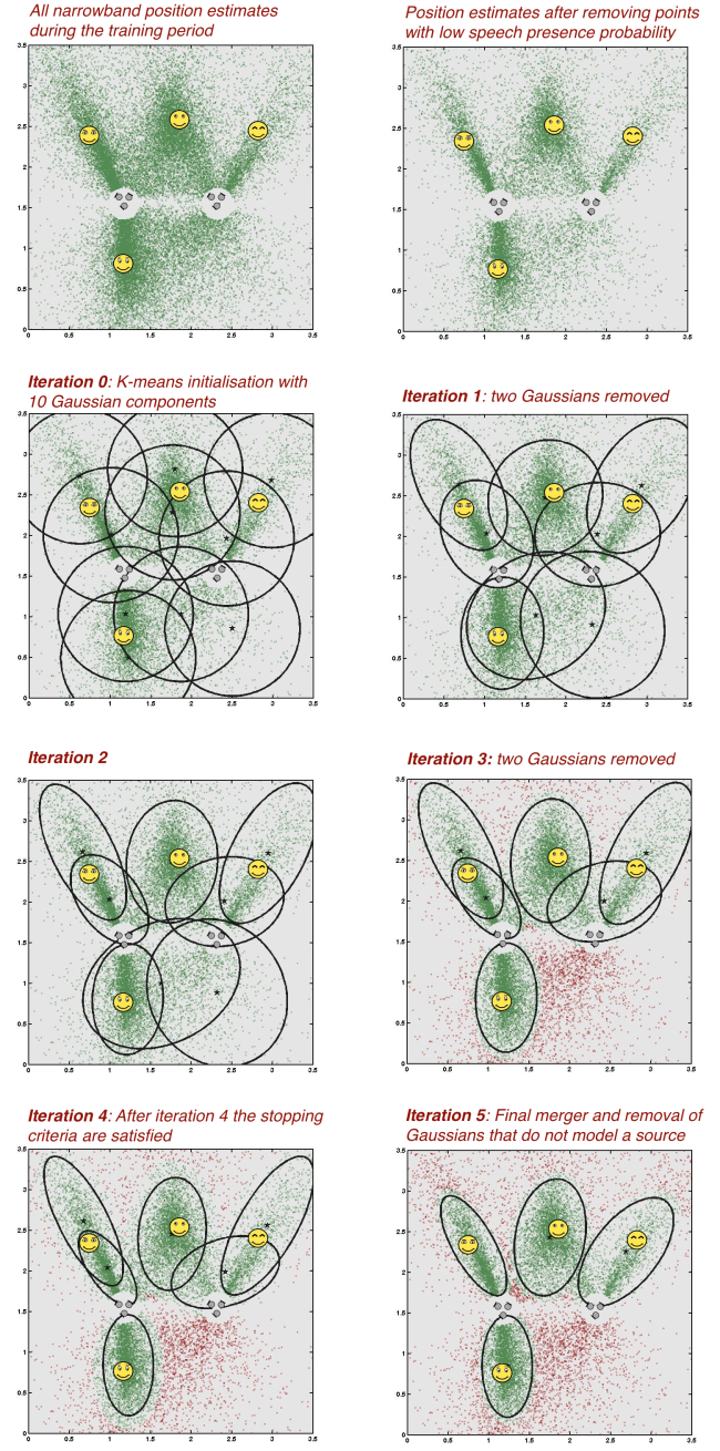
EXAMPLE 2
Four simultaneously active sources are captured by the microphones. The signal-to-noise was 10 dB and training was performed on an 8 seconds segment where all sources are active.
- Listen to the portion of the signal used for training by hitting the start button below.
- The iterations of the proposed EM-based algorithm for number of source detection and clustering.
- Listen to the separated signals and compare them to the mixture received at one of the microphones.
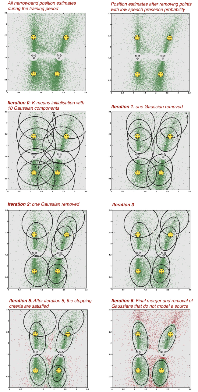
EXAMPLE 3
In this example, we show a four-sources scenario, with a different arrangement of the sources. Similarly as in Example 2, the training is performed on 8 seconds segment, however, in this case, the sources are not concurrent during training, and each source is active only 2 seconds. Note: This is still an unsupervised problem. Although each source has a separate period of activity during training, the EM algorithm determines clusters using the 8 seconds signal segment with unlabelled data.
- Listen to the portion of the signal used for training by hitting the start button below.
- The iterations of the proposed EM-based algorithm for number of source detection and clustering.
- Listen to the separated signals and compare them to the mixture received at one of the microphones.